Stock and flow diagram
Contents
Definition
A Stock & Flow Diagram (SFD) is similar to a Causal Loops Diagram (CLD) though provides a more rigourous representation. Both diagrams belong to the chapter System Dynamics. System dynamics is an approach to understanding the behaviour of complex systems over time. It deals with internal feedback loops and time delays that affect the behaviour of the entire system. What makes using system dynamics different from other approaches to studying complex systems is the use of feedback loops and stocks and flows. It depicts the structural understanding of a system - the causal structures that produces the observed behavior. It reveals information about the rates of change of system elements and the measures of the variables of the system.[1]
By explicitly identifying Stocks - reservoirs which change over time, and Flows, which are responsible for changes in Stocks, the resultant insight explicitly depicts the manner in which things change.
Stock & Flow Diagram i based on Causal Loops Diagram and captures:
- Stock
- Flows
- Quatified feedback loops
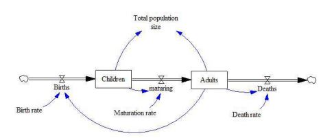
Example of Stock and Flow Diagram - Child-adult population model
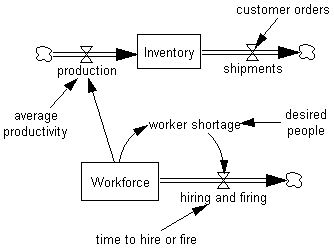
Shipments
Rules
- Stocks are always changed by flows
- In general, the formulas for the flows will depend on things that are changing (state)
Behaviour of model
System structure is defined by:
- Stocks
- Flows
- Connections between them
Nonlinearity: The behaviour of the whole is more than the sum of the behaviour of the parts
- Stock and flow structure (including feedbacks) of a system determines the qualitative behaviour modes that the system can take on
Symbols
Each graphical tool for modeling System Dynamics has its own form of symbols, but basics are same in the following points. [2] [3]:
Stocks
- In a stock & flow diagram are shown as rectangles
- Stocks (also known as Levels) represent accumulations
-– These capture the “state of the system”
-– Mathematically it can be called as “state variables”
- Are used to represent the real-world processes (e.g. stocks of material, knowledge, people, money)
- Stocks can be measured at one instant in time
- Stocks start with some initial value and are thereafter changed only by flows into & out of them
–- There are no inputs that immediately change stocks
- Stocks are the source of delay in a system
The Critical Role of Stocks in System Dynamics:
- Stocks determine current state of system
–- Stocks often provide the basis for making choices
- Stocks central to most disequilibria phenomena (buildup, decay)
- Lead to inertia
- Give rise to delays
Examples of Stocks
There is a list of common examples of Stocks:
- Water in a tub or reservoir
- People of different types
- Susceptible, infective,immune people
- High-risk individuals
- Healthcare workers
- Medicine in stocks
- Money in bank account
- CO2 in atmosphere
- Blood sugar
- Stored Energy
- Degree of belief in X
- Stockpiled vaccines
- Goods in a warehouse
- Beds in an emergency room
- Owned vehicles
Flows
All changes to stocks occur via flows. In turn, stocks in a system determine the values of flows.
- Drawn with an arrow with a valve (denoting the flow rate) in the middle of it
- Always expressed per some unit time: If these flow into/out of a stock that keeps track of things of type X (e.g. persons), the rates are measured in X/(Time Unit) (e.g. persons/year, $/month, gallons/second)
- Typically measure over certain period of time (by considering accumulated quantity over a period of time)
–- e.g. Incidence Rates is calculated by accumulating people over a year, revenue is $/Time, water flow is litres/minute
–- Can be estimated for any point in time
Examples of Flows
There is a list of common examples of Flows [x]:
- Inflow or outflow of a bathtub (litres/minute)
- Rate of incident cases (e.g. people/month)
- Rate of recovery
- Rate of mortality (e.g. people/year)
- Rate of births (e.g. babies/year)
- Rate of treatment (people/day)
- Rate of caloric consumption (kcal/day)
- Rate of pregnancies (pregnancies/month)
- Reactivation Rate (# of TB cases reactivating per unit time)
- Revenue ($/month)
- Spending rate ($/month)
- Power (Watts)
- Rate of energy expenditure
- Vehicle sales
- Vaccine sales
- Shipping rate of goods
Examples of Stock and flows
The following illustration shows the graphical implementation of symbols for one inflow to one Stock in software VenSim.
The following table provides examples of Stocks and their inflows and outflows
| Stock | Inflows | Outflows |
| bank balance | deposits interest | withdrawals |
| housing stock | housing investment | housing depreciation |
| CO2 in atmosphere | tons emitted | tons sequestered |
| population | births,
immigration |
deaths,
emigration |
| fuel tank | refueling | fuel consumption |
Cloud
Cloud represents either:
- Source of the flow - when the flow is originated from outside the model
- Sink of the flow - when the flow sinks
Both sources and sinks are assumed to have infinite capacity and do not impose any limitations on the flows. Clouds are drawn as the part of the flow element, in case the flow does not flows in/out of some stock.
Auxiliaries
Auxiliaries are used to define some intermediate concepts. Auxiliary can change instantaneously according to the specified formula.
Auxiliary variables are convenience names we give to concepts that can be defined in terms of expressions involving stocks/flows at current time
– Adding or eliminating an auxiliary variable does not change the mathematical structure of the system
- Critical for model transparency
– Can be reused at many places
– References to auxiliary variables prevents need for modeler to think about all of details of definition
- Enhanced modifiability: Single place to define
- Convenient for reporting (graphing, tables) & analyzing model dynamics
Parameters
Parameters are commonly used to define numeric constants.
Links
Link is used to define a dependency between elements of a stock and flow diagram.
If some element A is mentioned in the equation or initial value of element B, you should first connect these elements with a link going from A to B and only then type the expression in the properties of B.
Graphical representation
Graphs
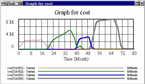
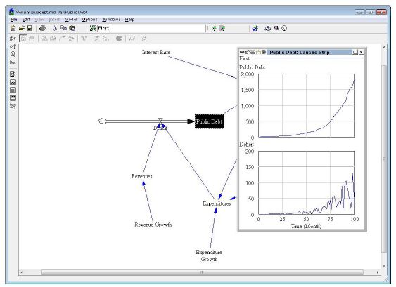
Each progress of simulation can be displayed into several charts that show the change in variables for example change in time. Once the simulation run is completed, you can look at the results of your simulation. The most basic and often most useful is the strip graph - See the following figure.
The time axis for the graph follows the global Start time and End time, but is rounded to even numbers. The Graph tool displays single or multiple variables on a single graph. It is useful for getting the big picture of a number of variables, and for printing presentation.
Each software tool for modeling the system dynamics allows you to set different settings for charts as a:
Graph Type (Normal, Cumulative, Stack) determines how data will be represented.
- Normal displays the values of the variables over time.
- Cumulative integrates the values of the variables. For positive variables, Cumulative yields an upward-sloping graph over time. The cumulation for a variable begins at the first time that values for the variable are available, regardless of the global Start time. This ensures that if you shorten the time range, the values will be the same as those in a graph of the full time range. Cumulative graphs allow you to view accumulations without adding additional model variables.
- Stack displays the values of the first variable normally, the second as the sum of the first and second variables, the third as the sum of the first three, and so on. All variables are stacked, including different subscript elements in a run and the same variable for different runs. For positive variables, this means that each successive variable is higher than its predecessors and that the final variable is the sum of all variables. An error occurs if the variables are from datasets with different sampling points (for example, different values of SAVEPER). Stack graphs are a convenient way of breaking down the components of a variable. It make the most sense to use stack graphs with one variable from multiple runs, or multiple subscripts from one run but rarely both.
The Table tool
The Table tool is very good tool, which is included for example in VenSim[5]. It can generate a read-only table that you can scroll to review values. The resulting table displays numerical values for variables and their causes or uses. The Table tool's most common use is for detailed analysis of a narrow time range, but it is also good for displaying a lot of values on the screen and also for displaying arrays of data at a given time.
Stats
The Stats tool is also included in VenSim[6] and it provides summary statistics on the Workbench Variable and its causes or uses. This tool provides a quick statistical overview of the values for a variable. The following figure shows the population statistics.
Software tools
There are a lot of software designed for modeling System Dynamics. An extensive list of programs can be found to be on this Wiki page. But the most used software are these:
Examples
Tutorial in VenSim
Task
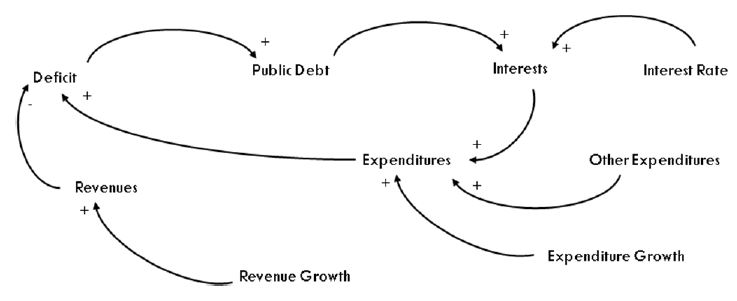
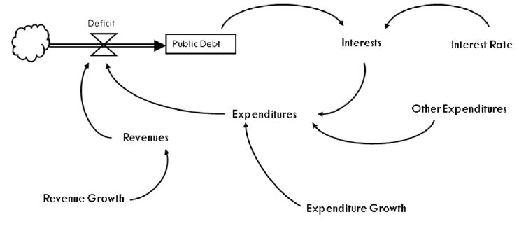
Convert the following model in the simulation environment VenSim.
Equations
- Deficit = Expenditures-Revenues
- Revenues= 300000 * RevenueGrowth
- Public Debt = INTEG(Deficit), initial value= 10
- InterestRate= RANDOM NORMAL(0.01, 0.1 , 0.05, 0.05,124)
- Interests= Public Debt* InterestRate
- RevenueGrowth= 0.02
- ExpenditureGrowth= 0.03
- OtherExpenditures= 200000
- Expenditures= Interests+OtherExpenditures* ExpenditureGrowth
Solution:
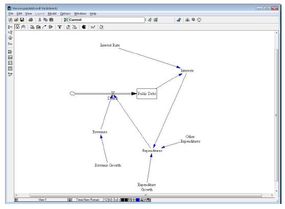
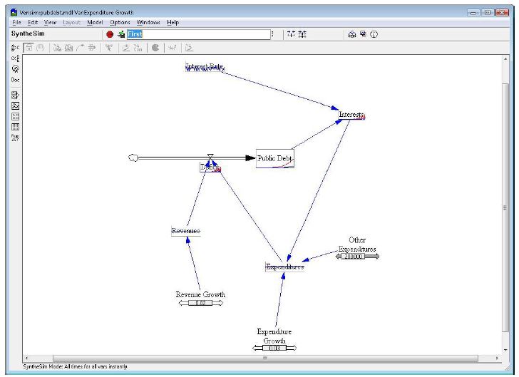
- Convert the Causal Loop Diagram (Figure 1) to the Stack Flow Diagram (Figure 2).
- Run Vensim. Click to create a new model. A window with the basic setup of the model appears - leave the default settings and press OK button.
- Click on Auxiliary variable, click on the screen and enter the variable name as "Revenues". The same way create any additional auxiliary variables depending on the model
- Click on Box variable, click on the screen and enter the name of the variable "Public Debt"
- Click on Rate, click on the screen and to variable "Public Debt" and name as "flow deficit" - thereby create material flow, which of infinite resources (cloud) outside the modeled system increases the variable "Public Debt"
- Click on Arrow, click on the source auxiliary variable and then to the target. This creates a flow of information. The same way create any additional auxiliary variables depending on the model
The following figure shows the final model:
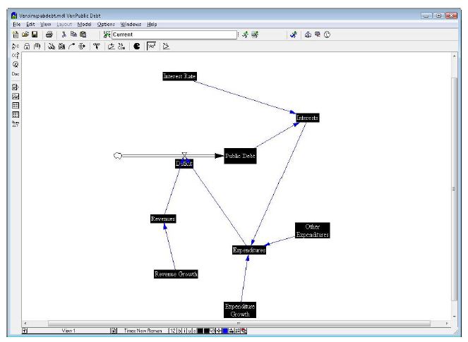
- Click on Equations button. This displays a mode for entering equations into individual variables. A variable which is not yet defined by the equation, is shown in black
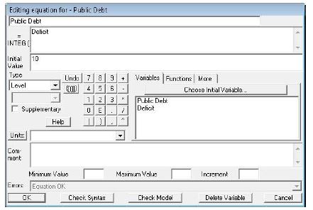
- Click on variable "Public Debt" and specify the initial state 10 (Equation 3). The formula for this variable is automatically supplemented by inflows to INTEG (Deficit)
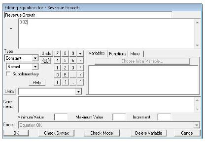
- Click on the variable "Revenue Growth" and enter the constant 0.02 (Equation 6). In the same way, enter the variable Expenditure Growth and Other Expanditures
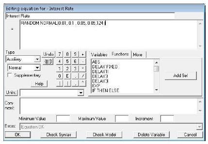
- A specific case is a variable "Interest Rate" that is not constant, but is randomly generated from a normal distribution (Equation 4). This function is used RANDOM NORMAL found on the Functions tab, along with other features that are available
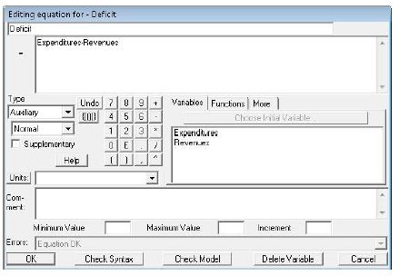
- Click on "Deficit" variable and enter the formula-Revenues Expenditures (Equation 1)
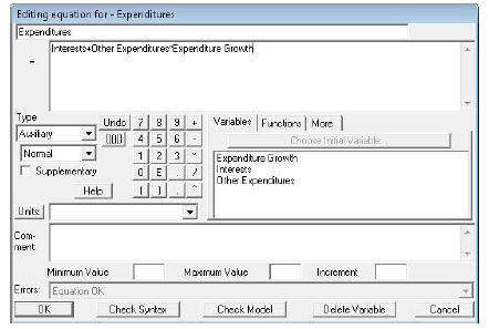
- Click on variable "Expenditures" and enter the formula "Interests + Other Expenditures * Expenditure Growth" (Equation 9). In the same way enter variables Revenues and Interests
- The simulation is started with the "Run a Simulation" button. The text box to the left of this button allows you to name the individual simulation runs.
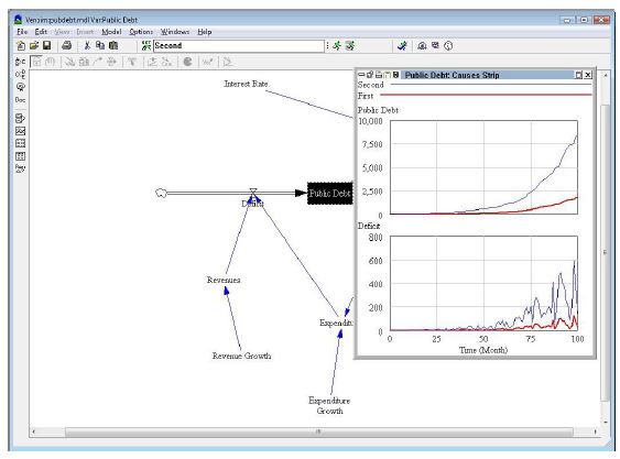
- We name the first run simulations as "First" and run a simulation. Then you can change the value of the variable "Expenditure Growth" to 0.03001, name running the simulation as a "Second" and again run the simulation
- The results of the simulation run can be displayed by clicking on the variable of "Interest", and then clicking to buttons Graph, or Causes Strip or Table to display the individual values. Each named running simulation is shown separately
- The simulation can be run in interactive mode.
- There is Automatical simulate on change button just next to the button Run a Simulation. This button starts interactive work with simulation, which allows you to interactively change the values of the input variables and immediately see the results of the change
Examples for practise
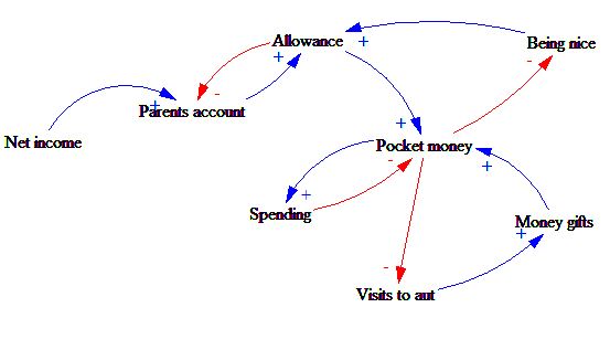
Pocket money
Try to convert following Casual Loop Diagram to Stock and Flow Diagram
A manufacturing firm
Create Casual Loop diagram, then convert it to Stock and Flow diagram:
A manufacturing firm maintains an inventory of finished goods from which it ships to
customers. Customer orders are filled after a delay caused by order processing, credit checks, etc.
Map the stock and flow structure, drawing on the following variables: Inventory, Raw Materials,
Production, Order Backlog, Order Rate.
Interests
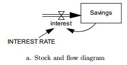
Create working simulation based on following proposal of Stock and Flow Diagram and equations.
Equations
- FINAL TIME = 40
- INITIAL TIME = 0
- interest = INTEREST RATE*Savings
- INTEREST RATE = 0.05
- SAVEPER = TIME STEP
- Savings = INTEG(interest,100)
- TIME STEP = 0.0625
Shipping delay
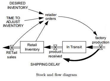
Create working simulation based on following proposal of Stock and Flow Diagram and equations.
Equations
- DESIRED INVENTORY = 200
- factory production = retailer orders
- FINAL TIME = 50
- In Transit = INTEG(factory production-orders received, 300)
- INITIAL TIME = 0
- product received = DELAY FIXED(factory production,SHIPPING DELAY, factory production)
- Retail Inventory = INTEG(product received-retail sales, 200)
- RETail sales = 100 + STEP(20, 5)
- retailer orders = retail sales+ (DESIRED INVENTORY- Retail Inventory) / TIME TO ADJUST INVENTORY
- SAVEPER = TIME STEP
- SHIPPING DELAY = 3
- TIME STEP = 0.0625
- TIME TO ADJUST INVENTORY = 2
References
- ↑ Stocks and flows diagram: Definition. CREATEADVANTAGE.COM. online
- ↑ Introduction to Stocks & Flows. OSGOOD, Nathaniel. INSTITUTE FOR SYSTEM SCIENCE & HEALTH. PDF
- ↑ Stock and Flow Diagrams: Stock and Flow diagramming notation. ANYLOGIC COM. online
- ↑ Vensim Help: Graph. VENTANA SYSTEMS, Inc. online
- ↑ Vensim Help: Table. VENTANA SYSTEMS, Inc. online
- ↑ Vensim Help: Stats. VENTANA SYSTEMS, Inc. online
