Time Series Model Building Process

Introduction

Linear time series models, e.g., ARIMA models for univariate time series, is a popular tool for modeling dynamics of time series and predicting the time series. The methodology is not popular only in statistics, econometrics and science, but also in machine learning business applications. The key question is how to build the model. We have to choose the form of the model, in particular number of lags for so-called autoregressive part (usually denoted as p) and moving average part of the model (usually denoted as d). The common guides usually provide a ‘cook book’ for model selection, see for example ARIMA Model – Complete Guide to Time Series Forecasting in Python . This goal of this simulation is to compare four basic methods for selection of lags (p) for the autoregressive part.

Problem Definition

The autoregressive process has form

Failed to parse (MathML with SVG or PNG fallback (recommended for modern browsers and accessibility tools): Invalid response ("Math extension cannot connect to Restbase.") from server "https://en.wikipedia.org/api/rest_v1/":): {\displaystyle x_t = {\mu} + {\phi}_1x_{t-1} + {\phi}_2x_{t-2}+...+{\phi}_px_{t-p} + {\epsilon}_t}

Failed to parse (MathML with SVG or PNG fallback (recommended for modern browsers and accessibility tools): Invalid response ("Math extension cannot connect to Restbase.") from server "https://en.wikipedia.org/api/rest_v1/":): {\displaystyle {\epsilon}_t \sim N(0,{\sigma}^2) }

However, we observe only the realized value and we do not know the hyperparameter p. Therefore, we must estimate it. The considered methods are following.

GETS (General-to-Specific)

We first start with high enough p (pmax in the code), and perform statistical test whether the last lag has statistically significant impact, i.e.,

Failed to parse (MathML with SVG or PNG fallback (recommended for modern browsers and accessibility tools): Invalid response ("Math extension cannot connect to Restbase.") from server "https://en.wikipedia.org/api/rest_v1/":): {\displaystyle H_0:{\phi}_p = 0}

Failed to parse (MathML with SVG or PNG fallback (recommended for modern browsers and accessibility tools): Invalid response ("Math extension cannot connect to Restbase.") from server "https://en.wikipedia.org/api/rest_v1/":): {\displaystyle H_0:{\phi}_p \neq 0}

If the impact is insignificant, we reduce p by one and continue until the parameter for the last lag is significant, i.e. last lag has significant effect.

Specific-to-General

The second approach works similarly as GETS, the only difference is that we first start with model without any lag, i.e.,

Failed to parse (MathML with SVG or PNG fallback (recommended for modern browsers and accessibility tools): Invalid response ("Math extension cannot connect to Restbase.") from server "https://en.wikipedia.org/api/rest_v1/":): {\displaystyle x_t = {\mu} + {\epsilon}_{t'}}

and we are adding lags until they are significant.

BIC (Bayesian Information Criteria)

Bayesian information criteria is based on a likelihood of the model and number of parameters. The criteria punish the model for high number of parameters for a potential over-fitting, and rewards the model for good fit of the data. The lower the BIC value is, the better the model (a little bit counterintuitive definition). We are supposed to select a model with the lowest value of BIC.

AIC (Akaike Information Criteria)

Works exactly the same as BIC, but the formula is slightly different.

Method and Simulation Method

The solution consists of three key elements, data generating process, AR(p) model, and simulation.

Data Generating Process

To answer the question, which model selection method is the best, we are generating an artificial data. We assume that data are created by AR(1) process

Failed to parse (MathML with SVG or PNG fallback (recommended for modern browsers and accessibility tools): Invalid response ("Math extension cannot connect to Restbase.") from server "https://en.wikipedia.org/api/rest_v1/":): {\displaystyle x_t = {\mu} + {\phi}_1x_{t-1} + {\epsilon}_{t'}}

or AR(2)

Failed to parse (MathML with SVG or PNG fallback (recommended for modern browsers and accessibility tools): Invalid response ("Math extension cannot connect to Restbase.") from server "https://en.wikipedia.org/api/rest_v1/":): {\displaystyle x_t = {\mu} + {\phi}_1x_{t-1} + {\mu} + {\phi}_2x_{t-2} + {\epsilon}_{t}}

with random error . Therefore, we must generate random numbers for random errors, and iterate over the equations described above. The initial values of the processes, e.g., Failed to parse (MathML with SVG or PNG fallback (recommended for modern browsers and accessibility tools): Invalid response ("Math extension cannot connect to Restbase.") from server "https://en.wikipedia.org/api/rest_v1/":): {\displaystyle x_0} , are set to the theoretical mean value of the process.

AR(p) model

For a given series Failed to parse (MathML with SVG or PNG fallback (recommended for modern browsers and accessibility tools): Invalid response ("Math extension cannot connect to Restbase.") from server "https://en.wikipedia.org/api/rest_v1/":): {\displaystyle {x_1,x_2,...x_T}} with a length T estimates a model for a given p.

Simulation

Perform n Monte Carlo simulations, where in each simulation the data generating process is used to create a time series. Then the AR(p) model is estimated for p=0,1,…,pmax, and the best models are selected according to the selection criteria described above. Therefore, we will obtain four estimates of p that corresponds to the described methods for each of the n simulation. The final step is to compute % success of correctly estimated p for each of four methods.

Controls

The solution allow to set number of simulation n. We need high enough n to make sure that the results will converge close enough to actual results. Therefore, we have set Failed to parse (MathML with SVG or PNG fallback (recommended for modern browsers and accessibility tools): Invalid response ("Math extension cannot connect to Restbase.") from server "https://en.wikipedia.org/api/rest_v1/":): {\displaystyle n=5000} . Higher n will not significantly increase the precision of the results.

The more important controls is selection of AR(1) or AR(2) process, and selection of parameters Failed to parse (MathML with SVG or PNG fallback (recommended for modern browsers and accessibility tools): Invalid response ("Math extension cannot connect to Restbase.") from server "https://en.wikipedia.org/api/rest_v1/":): {\displaystyle {\mu},{\sigma},{\phi}_1} and Failed to parse (MathML with SVG or PNG fallback (recommended for modern browsers and accessibility tools): Invalid response ("Math extension cannot connect to Restbase.") from server "https://en.wikipedia.org/api/rest_v1/":): {\displaystyle {\phi}_2} for the process. Additionally, we can set length of the generated series and even compare performance for series with two distinct lengths Failed to parse (MathML with SVG or PNG fallback (recommended for modern browsers and accessibility tools): Invalid response ("Math extension cannot connect to Restbase.") from server "https://en.wikipedia.org/api/rest_v1/":): {\displaystyle T_1} and Failed to parse (MathML with SVG or PNG fallback (recommended for modern browsers and accessibility tools): Invalid response ("Math extension cannot connect to Restbase.") from server "https://en.wikipedia.org/api/rest_v1/":): {\displaystyle T_2} . In other words, one method may perform better for low number of observations than other, and this control allow to compare the performance.

Results

• 

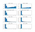
  Failed to parse (MathML with SVG or PNG fallback (recommended for modern browsers and accessibility tools): Invalid response ("Math extension cannot connect to Restbase.") from server "https://en.wikipedia.org/api/rest_v1/":): {\displaystyle {\Phi} = 0.1}

• 

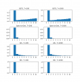
  Failed to parse (MathML with SVG or PNG fallback (recommended for modern browsers and accessibility tools): Invalid response ("Math extension cannot connect to Restbase.") from server "https://en.wikipedia.org/api/rest_v1/":): {\displaystyle {\Phi} = 0.9}

• 

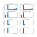
  Failed to parse (MathML with SVG or PNG fallback (recommended for modern browsers and accessibility tools): Invalid response ("Math extension cannot connect to Restbase.") from server "https://en.wikipedia.org/api/rest_v1/":): {\displaystyle {\Phi}_1= 0.4, {\Phi}_2 = 0.4}

• 

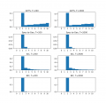
  Failed to parse (MathML with SVG or PNG fallback (recommended for modern browsers and accessibility tools): Invalid response ("Math extension cannot connect to Restbase.") from server "https://en.wikipedia.org/api/rest_v1/":): {\displaystyle {\Phi}_1= 0.0, {\Phi}_2 = 0.9}

Conclusion

Failed to parse (MathML with SVG or PNG fallback (recommended for modern browsers and accessibility tools): Invalid response ("Math extension cannot connect to Restbase.") from server "https://en.wikipedia.org/api/rest_v1/":): {\displaystyle {\phi} = 0.1}

Previous periods don't have big impact. AIC method works well with smaller samples. In case of bigger samples, BIC method works better than AIC.

Failed to parse (MathML with SVG or PNG fallback (recommended for modern browsers and accessibility tools): Invalid response ("Math extension cannot connect to Restbase.") from server "https://en.wikipedia.org/api/rest_v1/":): {\displaystyle {\phi} = 0.9}

BIC is the best method for small and big samples. Even though the GETS method doesn't work quite well, it is commonly used. The bigger tha max value of p is used, the bigger is the probability of getting the wrong guess from the simulation.

Failed to parse (MathML with SVG or PNG fallback (recommended for modern browsers and accessibility tools): Invalid response ("Math extension cannot connect to Restbase.") from server "https://en.wikipedia.org/api/rest_v1/":): {\displaystyle {\phi}_1 = 0.0} and Failed to parse (MathML with SVG or PNG fallback (recommended for modern browsers and accessibility tools): Invalid response ("Math extension cannot connect to Restbase.") from server "https://en.wikipedia.org/api/rest_v1/":): {\displaystyle {\phi}_2 = 0.9}

BIC is the best method for small and big samples again. As we can see, Spec-to-gen method gives us very wrong result in approximately 1/4 cases, because the null value gives no sense in this case.

Failed to parse (MathML with SVG or PNG fallback (recommended for modern browsers and accessibility tools): Invalid response ("Math extension cannot connect to Restbase.") from server "https://en.wikipedia.org/api/rest_v1/":): {\displaystyle {\phi}_1 = 0.4} and Failed to parse (MathML with SVG or PNG fallback (recommended for modern browsers and accessibility tools): Invalid response ("Math extension cannot connect to Restbase.") from server "https://en.wikipedia.org/api/rest_v1/":): {\displaystyle {\phi}_2 = 0.4}

This process is set to not be influenced by previous periods. The BIC method works the best again.

Code

Models.py

The part of the code 'class ARp(object)' was created with great help from another student and it is not originally created for this course.

import numpy as np from numpy.linalg 
import inv from scipy.stats 
import norm

def sim1(mu, phi1, sigmaSq, T):
    """
    Simulates single trajectory.
    :param mu:
    :param phi1:
    :param sigmaSq:
    :param T:
    :return:
    """
    x = np.zeros(T+1)
    epsilon = np.random.normal(0,sigmaSq, T+1)

    x[0] = mu / (1.0 - phi1)

    for t in np.arange(T):
        x[t+1] = mu + phi1 * x[t] + epsilon[t]

    return x[1:]

def trajectories1(mu, phi1, sigmaSq, T, n):
    """
    Simulates n-trajectories of AR(1) process
    :param mu:
    :param phi1:
    :param sigmaSq:
    :param T:
    :param n:
    :return:
    """
    X = np.zeros([n,T])
    for s in np.arange(n):
        X[s,:] = sim1(mu, phi1, sigmaSq, T)
    return X


def sim2(mu, phi1, phi2, sigmaSq, T):
    x = np.zeros(T+2)
    epsilon = np.random.normal(0,sigmaSq, T+2)

    x[0] = mu / (1.0 - phi1-phi2)
    x[1] = mu / (1.0 - phi1-phi2)

    for t in np.arange(T)+1:
        x[t+1] = mu + phi1 * x[t] + phi2 * x[t-1] + epsilon[t]

    return x[2:]

def trajectories2(mu, phi1, phi2, sigmaSq, T, n):
    """
    Simulates n-trajectories of AR(2) process
    :param mu:
    :param phi1:
    :param phi2:
    :param sigmaSq:
    :param T:
    :param n:
    :return:
    """
    X = np.zeros([n,T])
    for s in np.arange(n):
        X[s,:] = sim2(mu, phi1, phi2, sigmaSq, T)
    return X

class ARp(object):
    """AR(p) class allowing to estimate the model """

    def __init__(self, x, p, pmax):
        self.p = p
        self.x = x
        self.T = float(x.size)
        self.par = np.zeros(p+2) #np.array: c, phi_1, phi_2, ... phi_p, sigma^2

        #Init. matrices for OLS
        Y = self.x[pmax:]
        Xtemp = []

        for i in np.arange(Y.size):
            Xtemp.append(np.flip(x[i:(pmax+i)],0))
        X = np.ones((Y.size, p+1))
        X[:,1:] = np.array(Xtemp)[:,:p]

        #OLS Estimate
        Phi = np.dot(np.dot(inv(np.dot(X.T,X)),X.T),Y)
        SigmaS = np.sum((Y - np.dot(X, Phi))**2.0)/(self.T-pmax)
        self.par[:-1] = Phi[:]
        self.par[-1] = SigmaS

        #t-ratios
        self.VCOV = inv(np.dot(X.T,X))*SigmaS
        self.SE = np.diag(self.VCOV)**0.5
        self.t = self.par[:-1]/self.SE

        #likelihood and IC
        self.logL = (-(self.T-pmax)/2.0)*np.log(2.0*np.pi) + (-(self.T-pmax)/2.0)*np.log(SigmaS) + (-(self.T-pmax)/2.0)
        self.AIC = 2.0*((self.par.size)-self.logL)
        self.BIC = np.log(Y.size)*self.par.size-2.0*self.logL

Simulation.py

import numpy as np
import models as mod
import matplotlib.pyplot as plt
from scipy.stats import norm
##########################
#Simulation and settings
#########################
#general
pmax = 10 # Maximum number of lags
n = 5000 # Number of simulations
T1 = 200 # Length of the first time series
T2 = 2000 # Length of the second time series

#1. AR(1) process
#phi = 0.9
#mu = 5.0
#sigmaSq = 1.0
#X1 = mod.trajectories1(mu, phi, sigmaSq, T1, n)
#X2 = mod.trajectories1(mu, phi, sigmaSq, T2, n)

#2. AR(2) process
phi1 = 0.4
phi2 = 0.4
mu = 5.0
sigmaSq = 1.0
X1 = mod.trajectories2(mu, phi1, phi2, sigmaSq, T1, n) # Rows = individual series; columns = time periods
X2 = mod.trajectories2(mu, phi1, phi2, sigmaSq, T2, n)

#####
#GETS General to specific method
#####
tquantile = norm.ppf(0.95) #95% quantile


#T1 simulation
ARarray = []
tratiop1 = []
for i in np.arange(X1.shape[0]):
    p = pmax
    while True:
        ARtemp = mod.ARp(X1[i,:],p,pmax)
        if np.abs(ARtemp.t[-1]) < tquantile and p>0:
            p-=1
        else:
            ARarray.append(ARtemp)
            tratiop1.append(p)
            break
print "t-ratio T1 finished"
#T2 simulation
ARarray = []
tratiop2 = []
for i in np.arange(X2.shape[0]):
    p = pmax
    while True:
        ARtemp = mod.ARp(X2[i,:],p,pmax)
        if np.abs(ARtemp.t[-1]) < tquantile and p>0:
            p-=1
        else:
            ARarray.append(ARtemp)
            tratiop2.append(p)
            break
print "t-ratio T2 finished"

####################
#Specific-to-General
####################
tquantile = norm.ppf(0.95) #95% quantile


#T1 simulation
ARarray = []
tratiop1SOG = []
for i in np.arange(X1.shape[0]):
    p = 0
    while True:
        ARtemp = mod.ARp(X1[i,:],p+1,pmax)
        if np.abs(ARtemp.t[-1]) > tquantile and p<=pmax:
            p+=1
        else:
            ARarray.append(ARtemp)
            tratiop1SOG.append(p)
            break
print "t-ratio T1 finished"
#T2 simulation
ARarray = []
tratiop2SOG = []
for i in np.arange(X2.shape[0]):
    p = 0
    while True:
        ARtemp = mod.ARp(X2[i,:],p+1,pmax)
        if np.abs(ARtemp.t[-1]) > tquantile and p<=pmax:
            p+=1
        else:
            ARarray.append(ARtemp)
            tratiop2SOG.append(p)
            break
print "t-ratio T2 finished"

####################
#AIC and BIC
####################
#T1 simulation
AICp1 = []
BICp1 = []
for i in np.arange(X1.shape[0]):
    AICtemp = np.zeros(11)
    BICtemp = np.zeros(11)
    for p in np.arange(pmax+1):
        ARtemp = mod.ARp(X1[i,:], p, pmax)
        AICtemp[p] = ARtemp.AIC
        BICtemp[p] = ARtemp.BIC
    AICp1.append(np.argmin(AICtemp))
    BICp1.append(np.argmin(BICtemp))

print "T1 AIC+BIC finished"
#T2 simulation
AICp2 = []
BICp2 = []
for i in np.arange(X2.shape[0]):
    AICtemp = np.zeros(11)
    BICtemp = np.zeros(11)
    for p in np.arange(pmax+1):
        ARtemp = mod.ARp(X2[i,:], p, pmax)
        AICtemp[p] = ARtemp.AIC
        BICtemp[p] = ARtemp.BIC
    AICp2.append(np.argmin(AICtemp))
    BICp2.append(np.argmin(BICtemp))
print "T2 AIC+BIC finished"


####################
#Plot
####################

fig, axes = plt.subplots(nrows=4, ncols=2)
ax0, ax1, ax2, ax3, ax4, ax5, ax6, ax7 = axes.flatten()

ax0.hist(tratiop1, bins=11, range=(-0.5, 10.5), weights=np.zeros(n) + 1. / n)
ax0.xaxis.set_ticks(np.arange(0, 11, 1.0))
ax0.set_title('GETS, T=200')

ax1.hist(tratiop2, bins=11, range=(-0.5, 10.5), weights=np.zeros(n) + 1. / n)
ax1.xaxis.set_ticks(np.arange(0, 11, 1.0))
ax1.set_title('GETS, T=2000')

ax2.hist(tratiop1SOG, bins=11, range=(-0.5, 10.5), weights=np.zeros(n) + 1. / n)
ax2.xaxis.set_ticks(np.arange(0, 11, 1.0))
ax2.set_title('Spec-to-Gen, T=200')

ax3.hist(tratiop2SOG, bins=11, range=(-0.5, 10.5), weights=np.zeros(n) + 1. / n)
ax3.xaxis.set_ticks(np.arange(0, 11, 1.0))
ax3.set_title('Spec-to-Gen, T=2000')

ax4.hist(AICp1, bins=11, range=(-0.5, 10.5), weights=np.zeros(n) + 1. / n)
ax4.xaxis.set_ticks(np.arange(0, 11, 1.0))
ax4.set_title('AIC, T=200')

ax5.hist(AICp2, bins=11, range=(-0.5, 10.5), weights=np.zeros(n) + 1. / n)
ax5.xaxis.set_ticks(np.arange(0, 11, 1.0))
ax5.set_title('AIC, T=2000')

ax6.hist(BICp1, bins=11, range=(-0.5, 10.5), weights=np.zeros(n) + 1. / n)
ax6.xaxis.set_ticks(np.arange(0, 11, 1.0))
ax6.set_title('BIC, T=200')

ax7.hist(BICp2, bins=11, range=(-0.5, 10.5), weights=np.zeros(n) + 1. / n)
ax7.xaxis.set_ticks(np.arange(0, 11, 1.0))
ax7.set_title('BIC, T=2000')

fig.subplots_adjust(hspace=0.5)
plt.show()