A b test
Name: Sample size calculation for A/B test
Author: Vaso Dzhinchvelashvili
Method: Monte Carlo
Tool: Python
Contents
Some theory
A/B test is a test enabling to see how the feature influenced the performance (some target metric)
α (Alpha) is the probability of Type I error in any hypothesis test–incorrectly rejecting the null hypothesis
β (Beta) is the probability of Type II error in any hypothesis test–incorrectly failing to reject the null hypothesis. (1 – β is power).
Problem definition
Imagine you are the analyst and there is a real problem: you need to understand how many observations do you need, and how long should you conduct an experiment
Limitations
Normally, there are many experiments held within a same company, therefore, for a purity of an experiments, users should not be intersected (cannot participate in two different experiments at a same time) => longer you conduct an experiment, more experiments are getting postponed, therefore development of a product is stopped/slowed down.
So I hardcoded 3 months as a maximum length of an experiment, this way there is lower chance calculations will take an inappropriate time.
Let’s assume there is an ‘old’ feature, and ‘new’ feature is developed to replace the old one. The company needs to decide which feature should be used and which one should be sunsetted (exluded from the product). Both features cannot exist outside the experiment.
Goal
Your goal(as an analyst who uses the calculator) is to understand if a new feature is increasing/decreasing the target metric. You want an assumption to be statistically significant.
What you have
In real life situation there could be the following inputs:
1 Historical information on how users performed in the past for the old feature.
- Expectation of the metric
- Variation of the metric
2 How many users access the feature monthly
3 Also, you have some assumptions: you expect a new feature to increase/decrease the metric by 0-x% (both sides). Of course, you want your metric to skyrocket (+10000%) but in reality, you don’t expect more than, say, 20% raise. As mentioned, you can’t hold an experiment longer then 3 months. You might of course. But for the sake of evaluation of my work in somewhat appropriate time (calculation takes some time) I hardcoded the maximum length. But it could be changed in the code.
4 Lastly, there is some chance you are ready to take, to be wrong when assuming a difference was random/not random (i.e. because of a new feature) – normally 5%.
These parameters should be entered in the UI (how explained below)
Model
The calculator uses Monte Carlo method to calculate the chances to see a nonrandom difference in means for samples.
Also, the script uses 2 different formulas and 1 python function to calculate sample size needed to achieve some confidence level (as turned out, all the formulas are tuned for 80% accuracy, however, from the literature review it is not obvious where is a betta, as all the Z/T and other statistics have only alpha in the formulas).
How to run the simulation
1) Add UI-Copy1 clean file to a Jupiter notebook:

2) Run the first block of code:
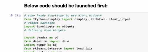

It should take not more then 20-30 seconds.
3) Run the second block of code:

It should also be launched pretty fast. As a result, the following UI should be visible. (I didn’t have to install any other software/libraries, but read on the internet someone had problems):

As it can be seen, all the parameters from the real life problem can be inserted to the calculator.
4) Please don’t brake the calculator intentionally: I tried to add all the required Catches of errors and suggestions on what can be fixed, but there is always a way to brake a code… The bigger monthly sample size is, the bigger is a calculation time. Now, pressing the button…
5) If there were no errors in the input, there is a timer-alike feature added, which will shed some light on how long is left for the calculations to finish.
![]()
Results
There are results of the simulation and results of the work (from a business point of view). First, we will see what is an actual outcome
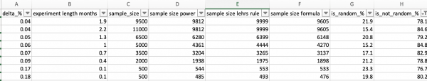
The result is the following. Here you can see what you can expect, if the delta is ±16% (both sides) and experiment held for 0.1… 1.3 months. For the line 153, 0.16% delta can be noticed in 1 month with 11% chance.


11% is low. Now analyst understands that either he should be expecting higher difference (which is hard to achieve by replacing 1 feature with another), or state to a product manager (owner of the feature) that there is no reason to conduct an experiment with existing limitations (monthly user flow, delta (expected difference)).
For the convenience the results are exported to out_ui.csv file, that can be found in the same repository where jupyter code was saved. For me it is in a root folder:

When downloading a file, the same table is visible, so it might be more convenient to navigate to the .csv file:

What else is exported:
Delta – expected difference. ‘what happens if the difference in metrics is 1%?’
Experiment length months – ‘what happens if we wait 0.1 month (first line)?’
Sample size – these many users will we get if we wait 0.1 month with a monthly flow of 100 users (note, users are divided equally into two groups, so if there is 100 monthly user flow, there will be 50-50 users in both groups).
Sample size power: how many users do we need according to pyhton function, if we need to detect 1% difference (and have some variation)
Sample size Lehr’s rule: How many users do we need according to Lehr’s rule of thumb to detect 1% difference.
Sample size formula: How many users do we need according to statistical formula from the article to detect 1% difference.
Is random= 1 – is not random – what is a chance we will notice the difference in 0.1 month if the real difference in means is 1% (3.9% chance for the first line – really low)
Conclusions (business point of view)
1) All formulas give pretty much the same number of users. So any of them can be used.
2) All formulas AND simulation display same number of users when it is 80% chance to detect a difference. That means, standard betta =20% is used in all the formulas. Here is how I know that: For the same parameters but monthly flow of 10 000 users (any huge number), the csv file generated the following statistics:

Here we can see that when last column (chance of detection of non random difference) is close to 80%, all formulas give pretty much the same sample size.
In case you run a test for Facebook, monthly users of the feature can be far more then 10k.
3) Formulas can be used only if you are satisfied with 20% chance of not detection. Otherwise, you should either be a good mathematician to be able to theoretically create a formula for a sample size to achieve, say, 95% chance of detecting a difference. OR you can just use my calculator, which is easier. Which I think is really something noone did before
Code
Code, explanatory letter and examples of generated CSVs File:Archive sim.zip
Literature
https://stats.stackexchange.com/questions/11131/sample-size-formula-for-an-f-test