Discrete event simulation
Contents
Introduction
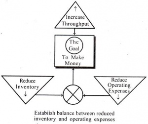
A few years ago Eliyahu Goldratt visited Alcatel Bell Telephone Manufacturing in Antwerp. Nowadays the company is part of Alcatel-Lucent Bell. The purpose of the visit was to discuss the company’s profitability issues. In a meeting with the management of the company his first question was: “What is the goal of your manufacturing organization?” Several ideas and opinions were brought up by the members of the management. The only answer that everybody agreed upon was: “The goal of a firm is to make money and be profitable”. Without that goal a company’s existence is in danger. There are several financial tools for the Chief Financial Officer to measure this goal. The most important are net profit, return on investment and cash flow. But how can a Chief Operation Officer decide and act in order to improve these financial goals? Goldratt answers this question with his Theory of Constraints.
He defines a series of operational measures:
- Throughput: is the rate at which a system generates money through sales or any other type of selling activities.
- Inventory: is the monetary value of the goods that are still in the system and which a company intends to use in its processes in order to sell their products.
- Operational Expense: is the monetary value of the expenses of the system in order to turn inventory into throughput.
Goldratt explains to the management that they should use these measures to reach the goal as follows: “Increase throughput while simultaneously reducing inventory and reducing operating expenses”
Accoring to Goldratt’s theory, constraints are the only limits of the system that keeps the company from reaching the goal. There are 5 steps that have to be executed in order to reach this goal.
- Identify the system's constraints.
- Decide how to exploit the system's constraints.
- Subordinate everything else to that decision.
- Elevate the system's constraints
- If in one the previous steps a constraint has been broken, go back to step 1.
The system’s constraints can also be defined as the bottlenecks in a system. The only way to improve the overall system is by process improvements at the bottlenecks. Finding these bottlenecks can be done using discrete-event simulations. A simulation can show hidden excess inventories, inefficiencies and overproduction. In the fourth step, the management makes the decision how to improve the bottlenecks. The consequences of these process changes can immediately be visualized and studied by a simulation of these improvements. These simulations give the possibility to quickly evaluate several solutions at a low cost. As a result, the management can choose the best possible solution. The improvement of Goldratt’s Theory Of Constraints and lean manufacturing in general, is just one of the many useful applications of discrete-event simulations. More applications and examples of discrete event simulations will be explained later in this chapter after we provided a solid definition and introduced the general ideas of discrete event simulations.
Definition
“Discrete event simulation utilizes a mathematical/logical model of a physical system that portrays state changes at precise points in simulated time. Both the nature of the state change and the time at which the change occurs mandate precise description. Customers waiting for service, the management of parts inventory or military combat are typical domains of discrete event simulation." [1]
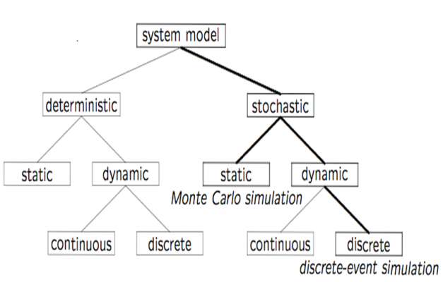
A more theoretical top-down description of discrete-event simulations is the following: The start of a discrete- event simulation is a model. A model is the construction of a conceptual framework, used to represent a system. The specific characteristics of discrete-event simulation model are the following:
- Stochastic: At least some of the models components are stochastic. This means that there is a certain factor of randomness in the model. This is represented by random number generators, which are explained in the terminology.
- Dynamic: The time evolution of the system’s components is important. Time is a significant variable.
- Discrete: The state of the system changes only significantly when events occur at discrete time instances.
The difference with continuous simulations is the use of the factor time. The system evolves over time so the variables change continuously in a continuous simulation. Whereas in a discrete event simulation the events itself determine if something happens or not. Time can go by without anything happening.
A combination of discrete and dynamic simulation is called a combined simulation. The basic is a continuous simulation but certain discrete events interfere the continuity of the simulation making it a combined simulation.
Monte Carlo simulations are static simulations. This means that the factor time is not a significant variable in this model, whereas time evolution is important when dealing with discrete-event simulations.
Terminology
Discrete-event simulations include the following important components:
Entities
Temporary entities are the elements that flow through the system. They wait in queues, follow a sequence of events and are specified by certain attributes. Most entities are introduced in a system according to a stochastic distribution. Examples of temporary entities are: parts of a good, customers and information messages.
Permanent entities remain in the system when the simulation is executed. They are used in the events to process the temporary entities. The usage time of permanent entities is mostly stochastically distributed. Examples of permanent entities are: operators, servers and machines.
Attributes
Entities own attributes that specify certain properties and states of the entity. They can affect how entities are handled during the sequence of the processes. They are not fixed through the flow so they can change by being processed. Examples of attributes are: priority and quality.
Events
Events change the state of the system. A sequence of events can be bundled as an activity. These events determine the timing and the flow of the simulation, hence the word discrete-event simulation. A typical example of an event is the arrival of new entity, often used to start the simulation. The sequence of events ordered by time of occurrence forms an event list. Each simulation has at least one event list. This events list determines the mechanism for advancing the simulation time. This sequence of actions is also called event-scheduling. Every simulation also needs a stopping event or ending condition. This determines how long the simulation will run. Typical stopping events are a specific time in the future or a condition that the simulation itself fulfills.
Queue
Place where temporary entities wait an undetermined time before being accepted in an event. Some entities might have priority attributes to skip the queue. These queues can for example be used to locate overproduction or a bottleneck as mentioned in the introduction.
State variables
These variables describe the system at different points in time. They change according to the processes in the events.
Clock
The clock maintains the simulation time. The measurement units vary depending on the characteristics of the model. Because we are dealing with discrete-events, the time is not continuous but “jump” according to the events. The clock is also responsible for the timer of the events.
Random number generators
Most of the previous components need the possibility to generate random variables in order to simulate the stochastic distributions. Pseudorandom number generators are used to accomplish this.
Statistics
The result of a simulation should be shown in the form of a report that gives statistics about all the important components of the discrete-event simulation. These statistics are analyzed to make better decisions.
How to solve a discrete event simulation
There is a general algorithm to solve a standard discrete-event simulation model. The algorithm consists of several steps and the process is typically iterative. The algorithm should be used many times in order to obtain the most optimal solution.
- Start with a real system and make sure you understand its characteristics. Determine the goals and objectives of the simulation. Why do we need the simulation? What problem do we have to solve? Answering these questions is essential to give meaning to the following steps.
- Design a model of the real-life system. Which variables and aspects of the system are relevant for the simulation? Are there any variables or aspects that can be ignored to simplify the model?
- Convert this model into a computational model that can be executed by a computer. When doing this an important aspect is the choice of the programming language. The two main possibilities are: a general-purpose programming language or a special-purpose simulation language. More information about these languages can be found in the Execution chapter.
- The last step in this general algorithm is the analysis of the output of the computational model. By doing this you can fully understand the nature of the real system and also predict the output when variables of the model change.
On top of this algorithm we need to verify and validate the simulation model. We need to check if the computational model is consistent with the real system. This additional process is done iteratively over the steps in the general algorithm to ensure the quality of the simulation.
Execution
The execution of the computational model is one of the most important issues when dealing with simulations. Generally there are two beliefs about how to solve this issue.
“For any important large-scale real application we would write the programs in a standard general-purpose language, and avoid all the simulation languages we know." [2]
On the other hand: “we believe, in general, that a modeler would be prudent to give serious consideration to the use of a simulation package." [3]
General-purpose programming languages
Discrete-event simulation is a particular application of scientific computing. Therefore most general-purpose programming languages are suitable for solving discrete-event simulations. Nowadays C, C++ and Java are the most commonly used languages because of their popularity amongst all programmers. The main advantage of general-purpose programming languages is the flexibility and freedom they offer to programmers.
Special-purpose simulation languages or simulation languages
These simulation languages are specially build to solve simulation problems. They have built-in tools that offer many components of discrete-event simulations. The main advantage of simulation languages is the decrease in programming time. Another advantage is the use of animations. These animations make the models easier to understand. Some examples of simulation languages are: Simul8, ProModel and GPSS.
Real applications
Al lot of industries and economic sectors use simulations. A brief summary of some real life applications is given here.
- In hospitals and healthcare in general, simulations are used for modeling waiting list of patients, modeling facility changes and bed planning.
- Banks and financial service firms use discrete-event simulations for the modeling and simulation of their call centers and for the cash management of ATM’s.
- The applications in logistics and transportation corporations are obvious: optimizing the material handling system, manpower planning and shipping strategies.
- The public sector including the police and the army uses discrete-event simulations for the modeling of emergency cases and the engineering of criminal investigation process.
Solved example
Airline companies often have a telephone reservation system. In order to optimize this system we need to do a discrete-event simulation. The goal of this model is to simulate the effectiveness of the system with a different number of reservationists. The model can be described as follows:
The customers can only make a reservation by telephone, so all customers have to call on the phone. Customers will not hang up so a customer can wait an indefinite amount of time. There is an unlimited amount of costumers that can be waiting on the phone at the same time. A new customer will get a 9-seconds recorded message in case all the reservation employees are busy. There are M reservationists working to answer the customer’s reservation needs. The incoming calls follow an exponential distribution and occur at a rate of λ. Customers can have two types of requests. First of all a flight reservation that requires multiple-destinations with probability p and secondly a single-destination flight reservation with probability 1-p. The service time of a multiple-destination request follows a log-normal distribution with mean μ and standard deviation σ. The service time of a single-destination request follows a Weibull distribution with shape k and scale λ. The overall probability distribution of service time is a combined density function based on the probability and the distribution of the two options.
We can solve this problem in the following steps:
- We start with a real system as described above. Our goal is to simulate the performance of the reservation system with a different number of reservationists.
- Secondly we need to design a model of this real-life system. In order to do that properly we need to define the entities and their attributes with possible values and the events and their sequence.
- Convert this model into a computational model that can be executed on a computer.
- Analyze the report of the computational model
The result for our entities and their attributes with possible values is the following:
- Customer (Entity):
- Reservation Type (Attribute):
- Single-Destination (Value)
- Multiple-Destination (Value)
- Status (Attribute):
- Listening 9-seconds message (Value)
- Waiting for service (Value)
- Getting service (Value)
- Reservation Type (Attribute):
- Reservationist (Entity):
- Status (Attribute):
- Idle (Value)
- Busy (Value)
- Status (Attribute):
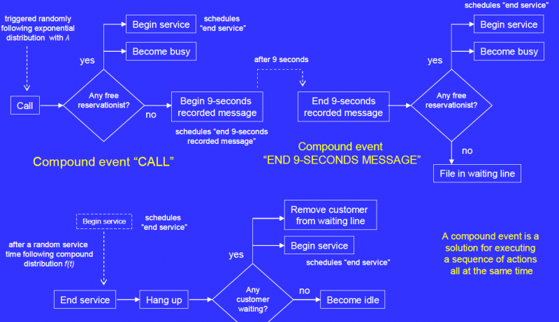
The events for this simulation are:
- Call (start) (customer)
- Hang up (end) (customer or reservationist)
- Begin service (customer or reservationist)
- End service (customer or reservationist)
- Begin 9-seconds recorded message (customer)
- End 9-seconds recorded message (customer)
- File in waiting line (customer)
- Remove customer from waiting line (reservationist)
- Become busy (reservationist)
- Become idle (reservationist)
Exercises
These excercise will help you to make your first simulation.
Building conceptual model
In order to fully understand how to build a conceptual model of a discrete-event simulation you should try to build a simple one yourself. Solve step 1 and 2 of “How to solve a discrete event simulation” of the following problem. At the post office there is one employee serving customers. Customers arrive according to an exponential distribution and occur at a rate of λ. The service time follows a log-normal distribution with mean μ and standard deviation σ. If the post employee is not working the customers start queuing. The customers will wait an infinite amount of time if necessary. What would happen if there would be a second employee serving customers? If you have solved this correctly you should find something like this:
- Our goal is to simulate system with extra employee. What is going to happen to our queue?
- The entities and events should be:
- Customer (Entity):
- Status (Attribute):
- Waiting in queue (Value)
- Getting service (Value)
- Status (Attribute):
- Employee (Entity):
- Status (Attribute):
- Idle (Value)
- Busy (Value)
- Status (Attribute):
The events of the system are:
- Arrival (start) (customer)
- Departure (end) (customer or reservationist)
- Begin service (customer or reservationist)
- End service (customer or reservationist)
- Queue (customer)
- Get out of queue (reservationist)
- Become busy (reservationist)
- Become idle (reservationist)
If you add specific variables and values you are ready for exercise 2!
Computational model
When you have your conceptual model ready, the next step is to execute the model in a computer program. There are two different types that are mainly used to do this. Can you name these two and explain them briefly and give advantages and disadvantages?
With the information you gained in this exercise you can decide for yourself which kind of program you prefer. You can now download or buy this program and practice translating the conceptual model from exercise 1 in a computational model. Use several values and for each variable and see what happens. Learn by trial and error to understand how the system works. Try to analyze the reports and make a decision based on that report.
If you have followed all of the above steps, you just generated your first reports and made a decision that was enforced by a discrete-event simulation. You are ready to solve more difficult problems and to become a real simulation engineer!
References
- ↑ Nance, Richard E.(1993). "A History of Discrete Event Simulation," Virginia Poltechnic Institute and State University
- ↑ Bratley P, Fox B. L., Schrage L. E. , (1987). "A Guide to Simulation, " Springler-Verlag, New York
- ↑ Law M. A., Kelton K. W., (2000). "Simulation Modeling and Analysis", McGraw-Hill Education
- http://www.albrechts.com/mike/DES/index.html
- http://eprints.cs.vt.edu/archive/00000363/01/TR-93-21.pdf
- http://parallel.vub.ac.be/research/pdes/supermarket_model.html
- http://coins.csrlab.org/imamu/akoubaa/cs433/Textbooks/Discrete%20Event%20Simulation%20-%20A%20First%20Course%20-%20Lemmis%20Park.pdf
- http://unitedbiosource.com/scientific/health-economics/discrete-event-simulation.aspx
- http://arrow.dit.ie/buschmanrep/3/
- http://www.vrtuosi.com/OAM/VR_MAD001/VRTUOSI_Simulation_Chapter_4a.pdf
- http://www.caciasl.com/cust_center/ss3docs/contin.pdf


